Water on the Landscape of the Pre-Columbian Bolivian Amazon
Abstract
This project examines the interaction between water and the landscape of the Pre-Columbian Bolivian Amazon, specifically how this landscape was seasonally flooded and how earthworks were used by the precolumbian inhabitants of the region to capture, manage, and retain floodwater for use in transportation, communication, fishing, and agriculture. To visualize this dynamic waterscape, a mesh of the landscape was built and used in a realistic physical water simulation. Using relevant archaeological, ethnographic, and historical literature and photographs of the earthworks and local environment, a timelapse animation of the landscape was created to show the cycle of inundation.
Figures
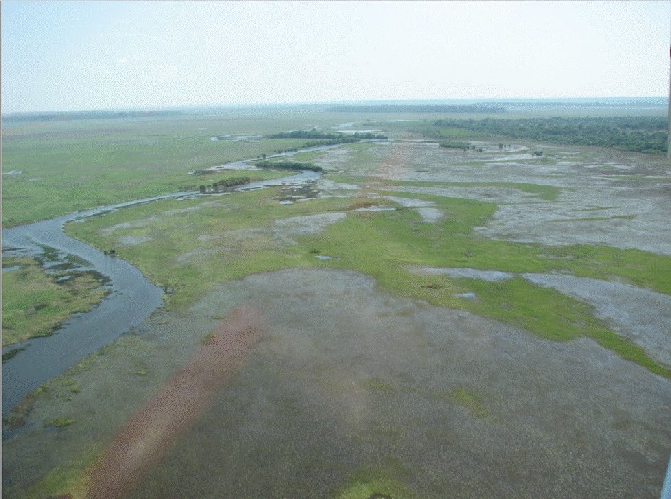
Figure 1: Photograph showing partially inundated savanna in Baures, Bolivia (Erickson et al. 2018a:Figure 6).
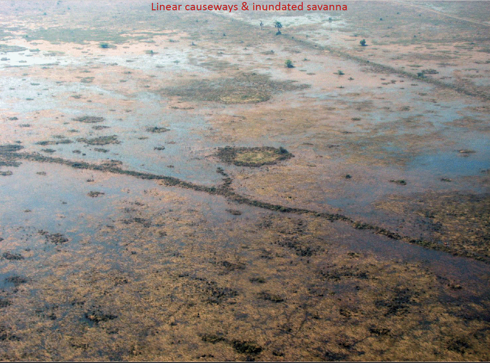
Figure 2: Photograph showing linear causeways crossing an inundated savanna (Erickson et al. 2018a:Figure 14).
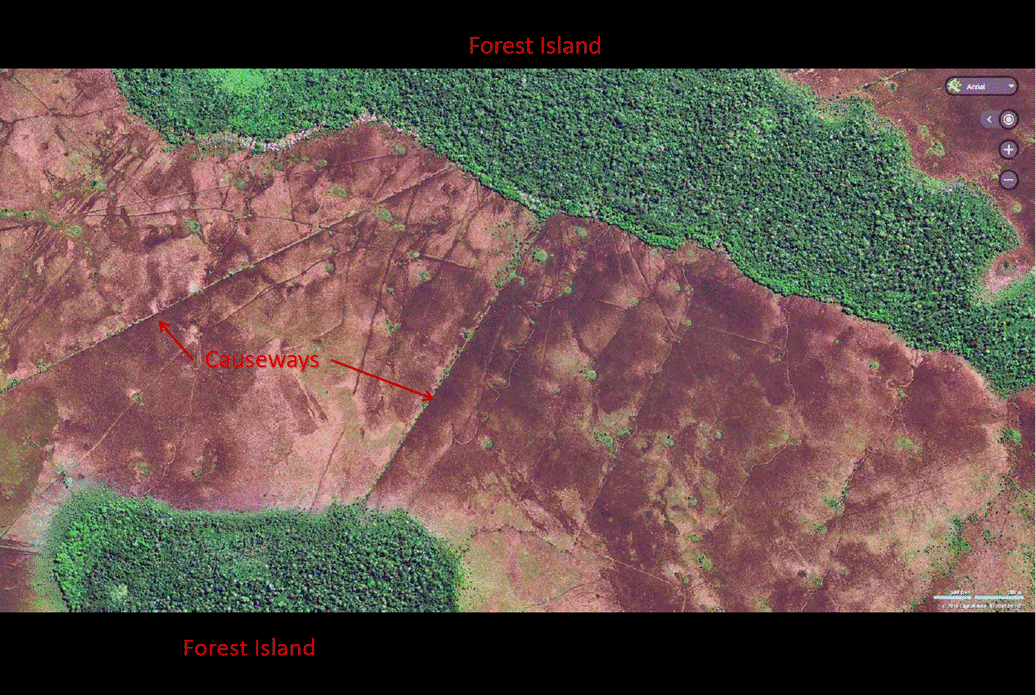
Figure 3: Principle reference for landscape model: satellite imagery showing forest islands and causeways (Erickson et al. 2018a:Figure 11).
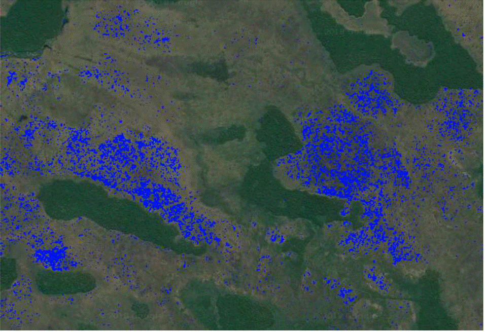
Figure 4: Sentinel 1 mapping of water extent from April 2017 superimposed on imagery from Google Earth containing the modelled region (Erickson et al. 2018b:46 Figure 28).
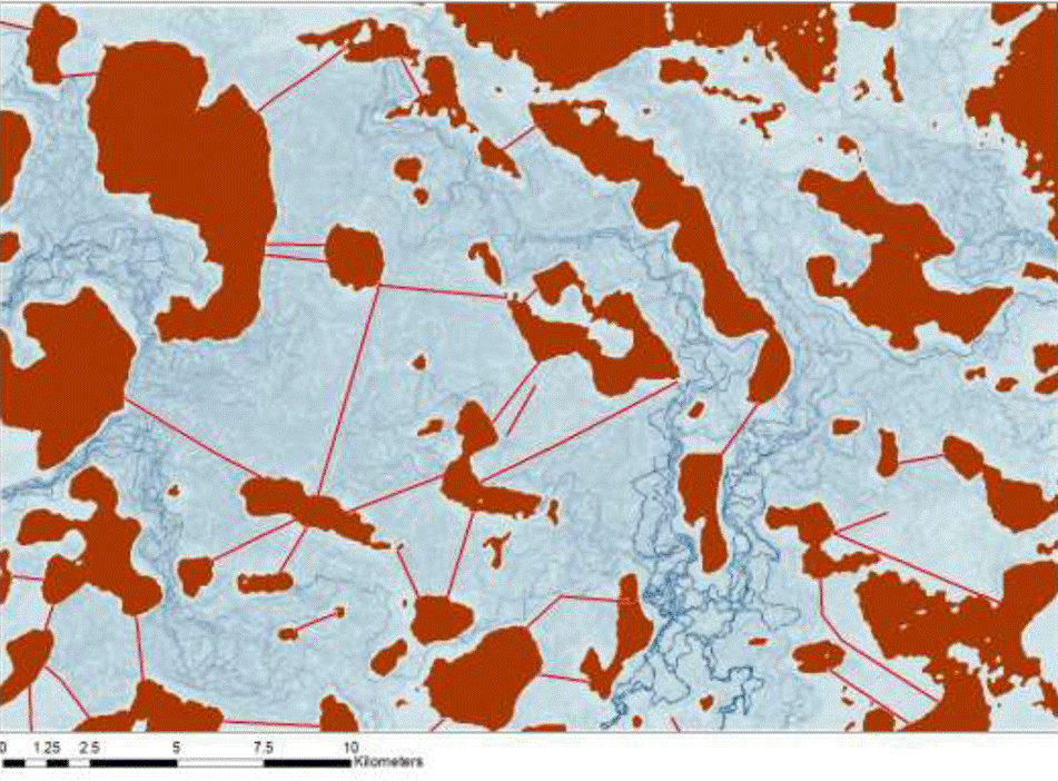
Figure 5: Natural Landscape Model (NLM) showing 20 iterations of Successive Flow Accumulation on a subset of landscape containing the referenced region (Erickson et al. 2018b:42 Figure 22).
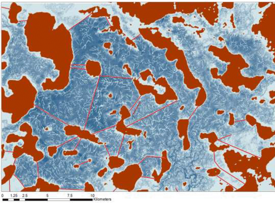
Figure 6: Natural Landscape Model (NLM) showing 100 iterations of Successive Flow Accumulation on a subset of landscape containing referenced region (Erickson et al. 2018b:42 Figure 23).
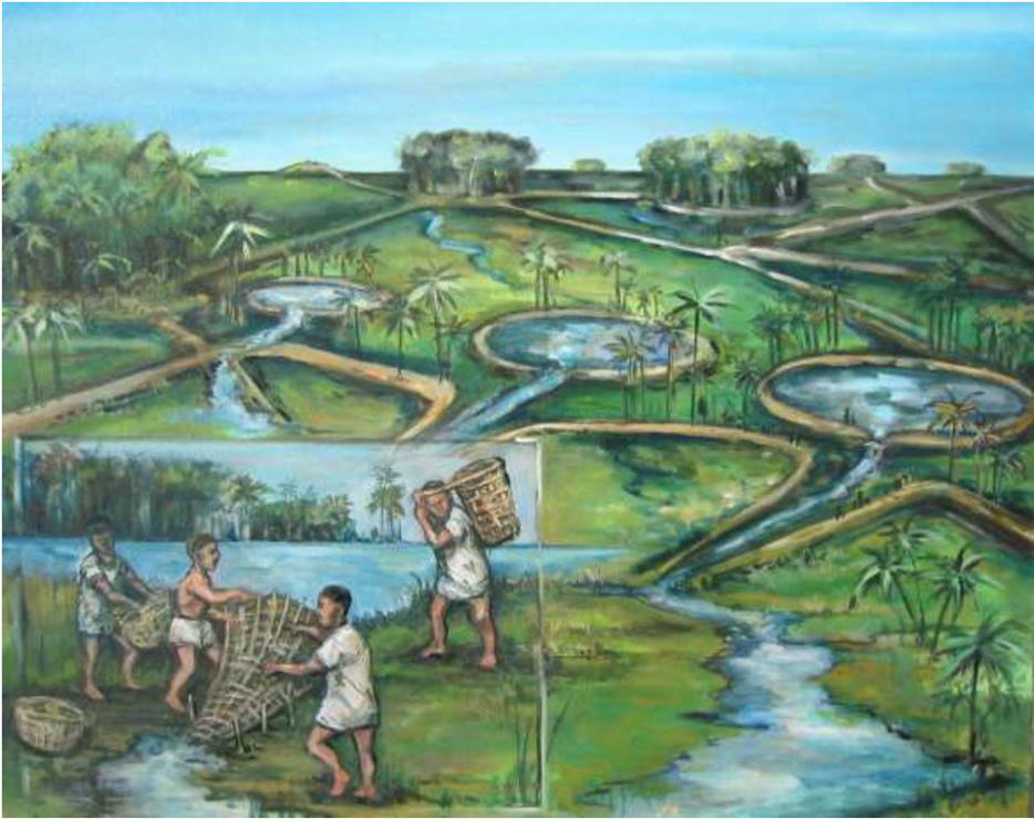
Figure 7: Artistic reconstruction by Dan Brinkmeier of pre-Columbian fish weirs and ponds (Erickson et al. 2018b:37 Figure 9).
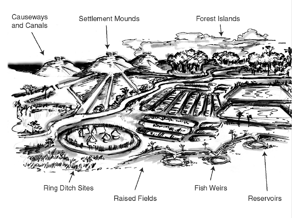
Figure 8: Labelled artistic reconstruction by Dan Brinkmeier of pre-Columbian earthworks of the Bolivian Amazon (Erickson 2018:Figure 25).
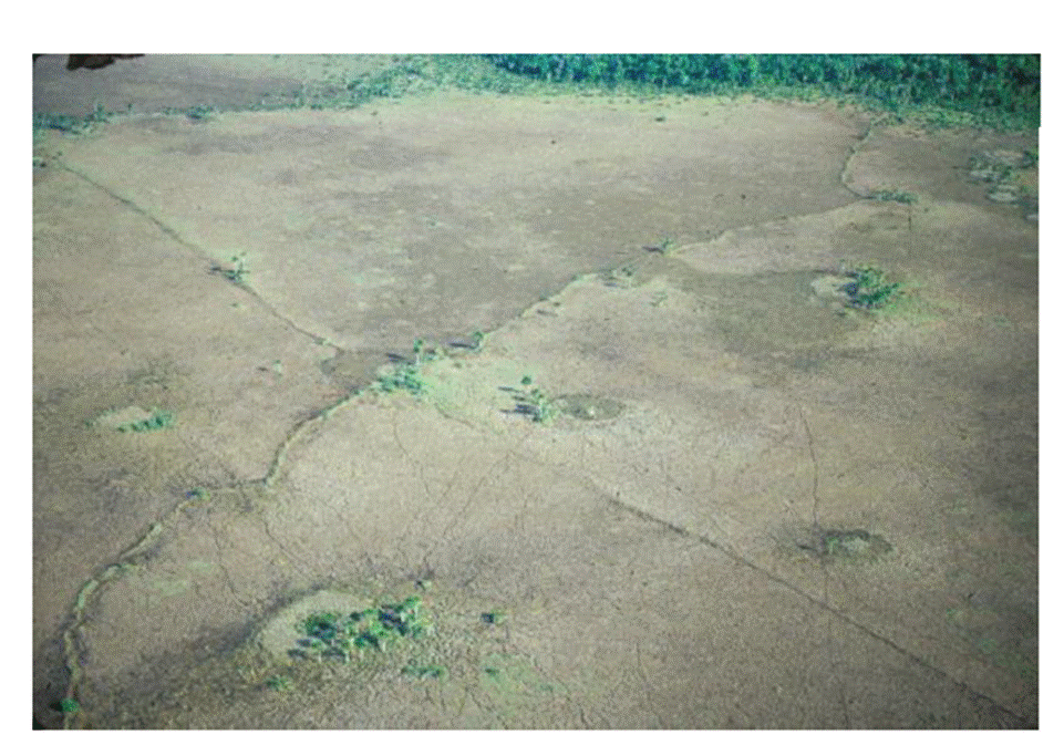
Figure 9: Pre-Columbian fish weirs and fish ponds on the savanna landscape of Baures (Erickson et al 2018:Figure 61b).
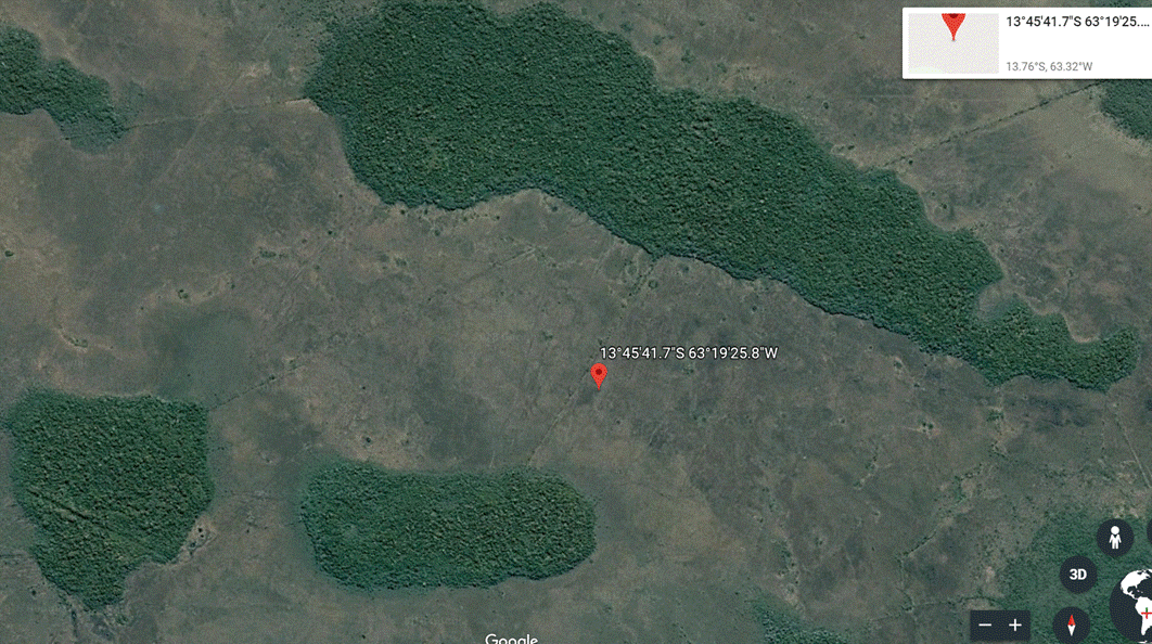
Figure 10: Satellite imagery of region referenced for landscape model (Google Earth 7.3.2, 2018. Bolivian Amazon 13º45’41.65” S, 63º19’25.82”W, elevation 150M. [online] Available through: https://earth.app.goo.gl/7h52pa [Accessed 7 December 2018]).
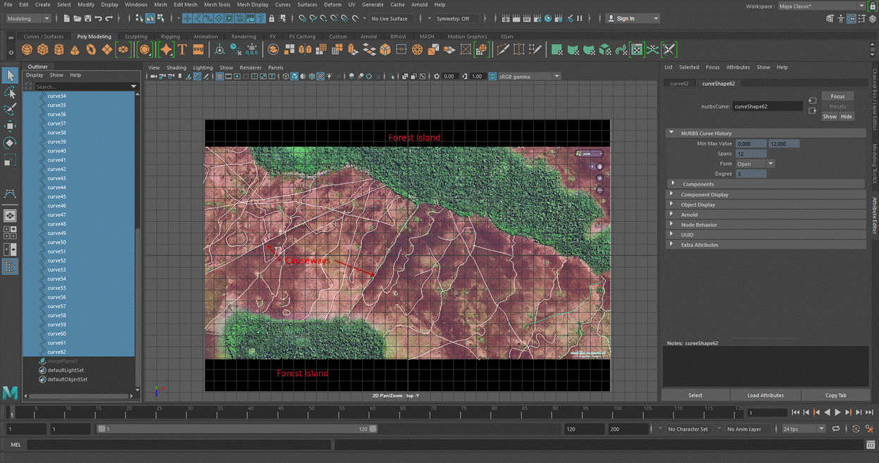
Figure 11: Digitized causeways and fish weirs of the sample landscape of the Bolivian Amazon
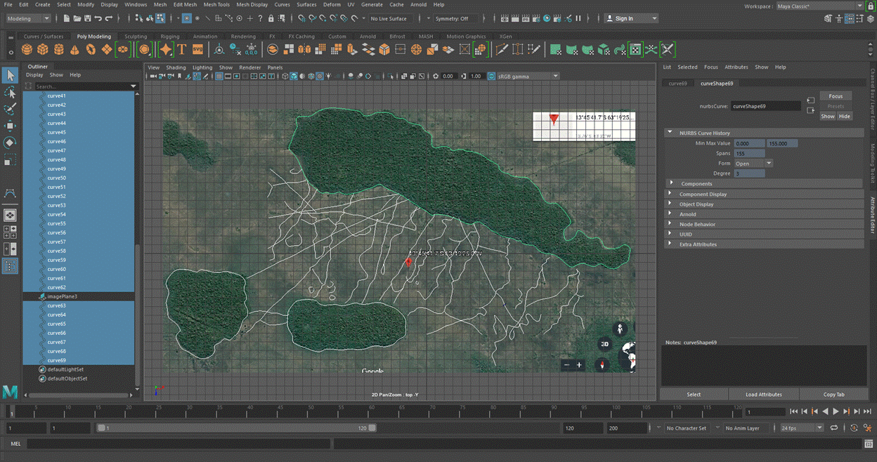
Figure 12: Digitized forest islands of the sample landscape of the Bolivian Amazon
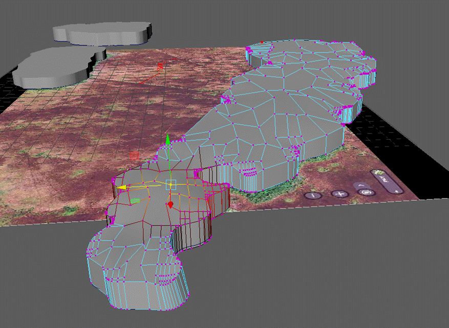
Figure 13: Extruding and modeling a forest island in Maya.
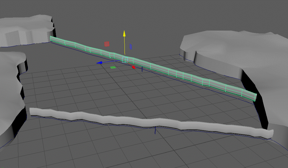
Figure 14: Extruding and modeling causeways between forest islands in Maya.
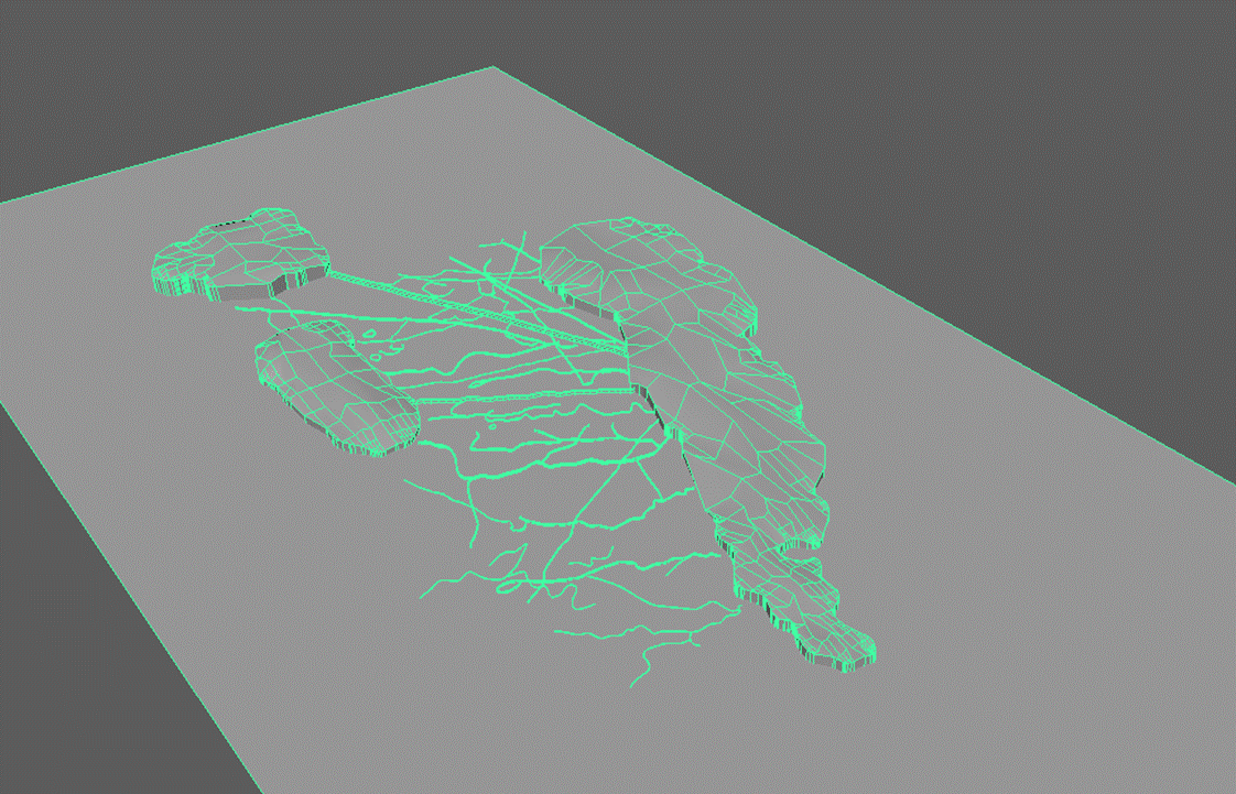
Figure 15: Forest islands and network of earthworks on the landscape modeled in Maya
Figure 16: Preparing causeways, fish weirs, and forest islands for nCloth simulation
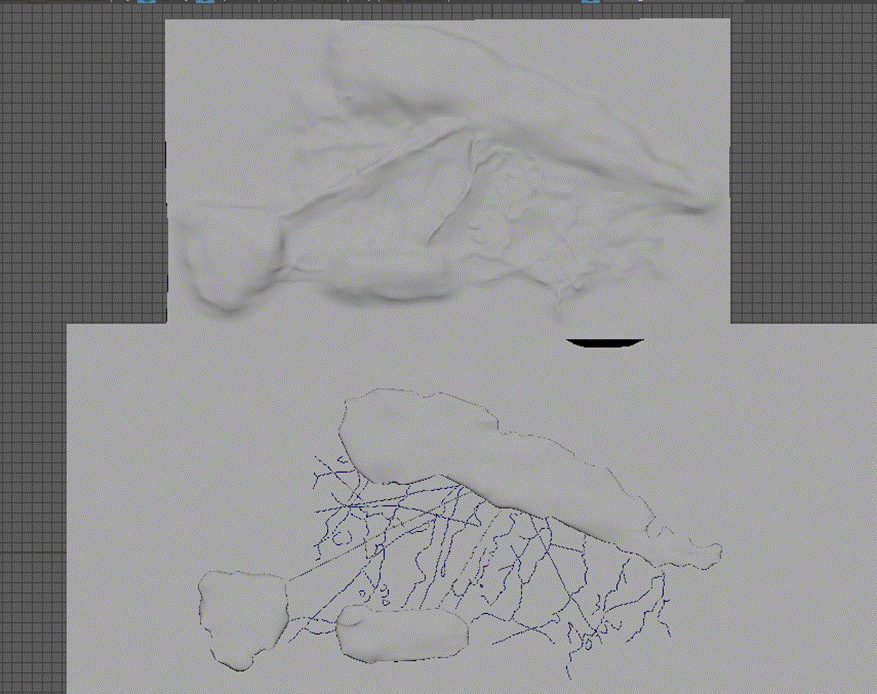
Figure 17: Result of nCloth simulation on forest island and earthwork passive colliders.
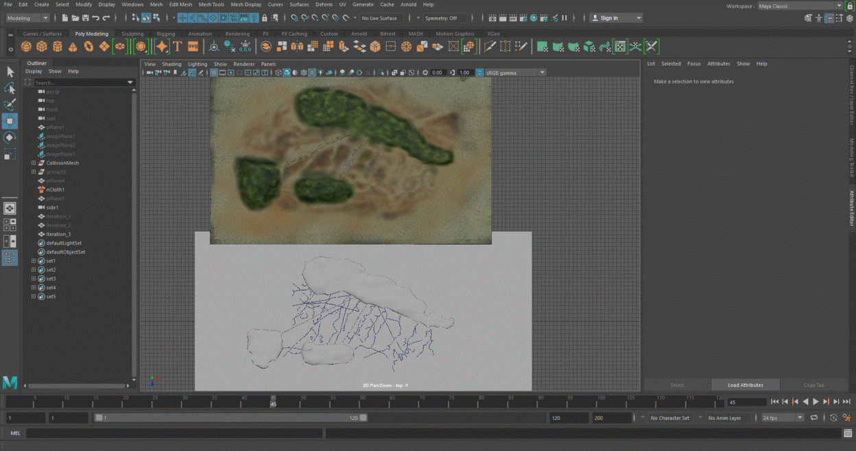
Figure 18: Initial texturing landscape mesh in MudBox.

Figure 19: Final landscape mesh with color and bump maps in MudBox.

Figure 20: Camera set-up in Houdini.
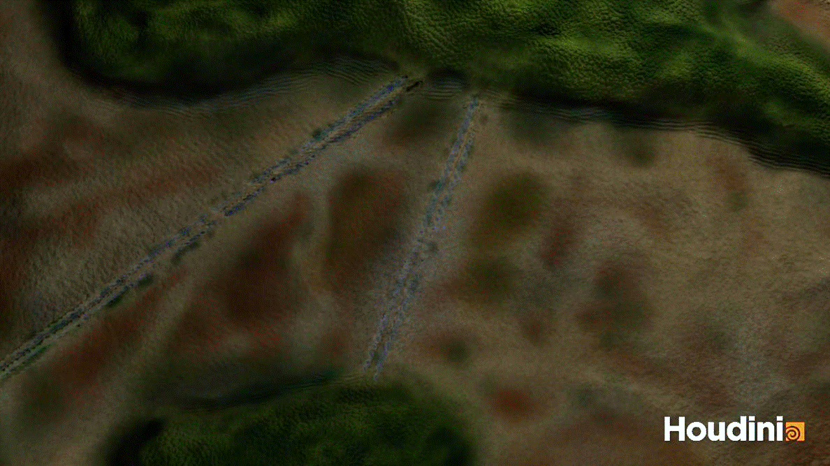
Figure 21: Camera 1 Position

Figure 22: Camera 2 Position

Figure 23: Initial fluid container set-up in Houdini.
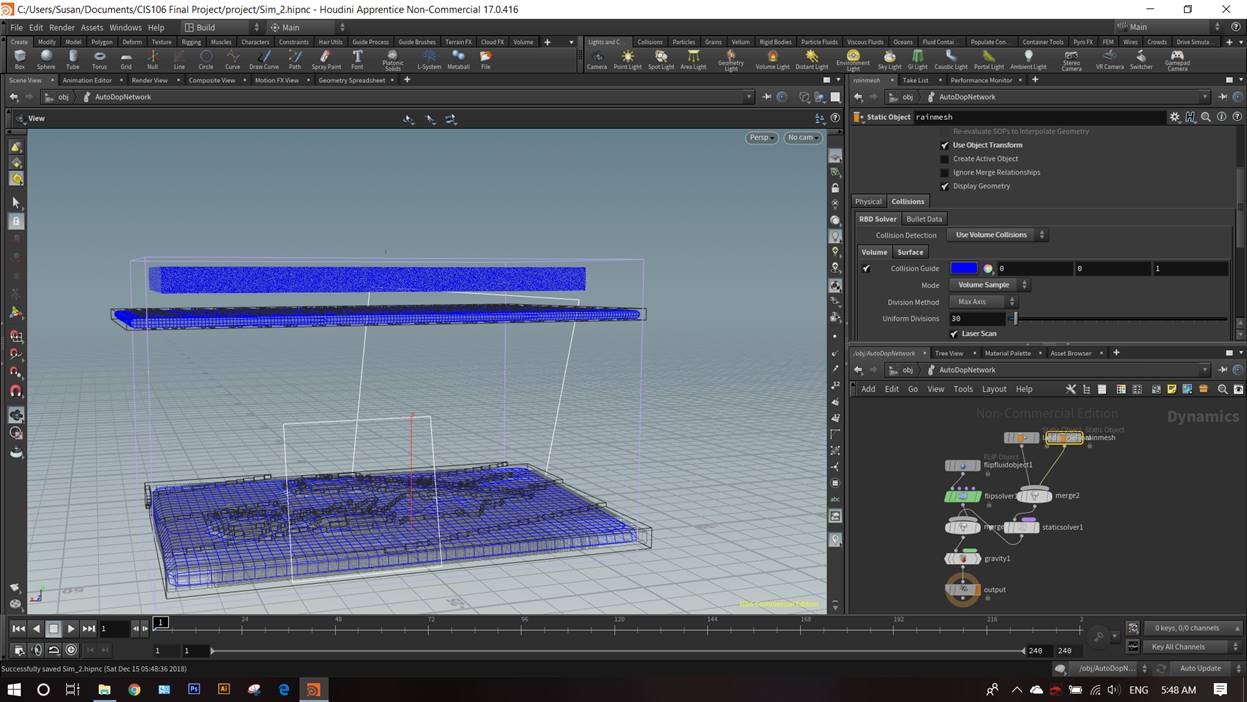
Figure 24: FLIP fluid rain simulation attempt in Houdini.
Figure 25: Failed FLIP fluid simulation attempt.
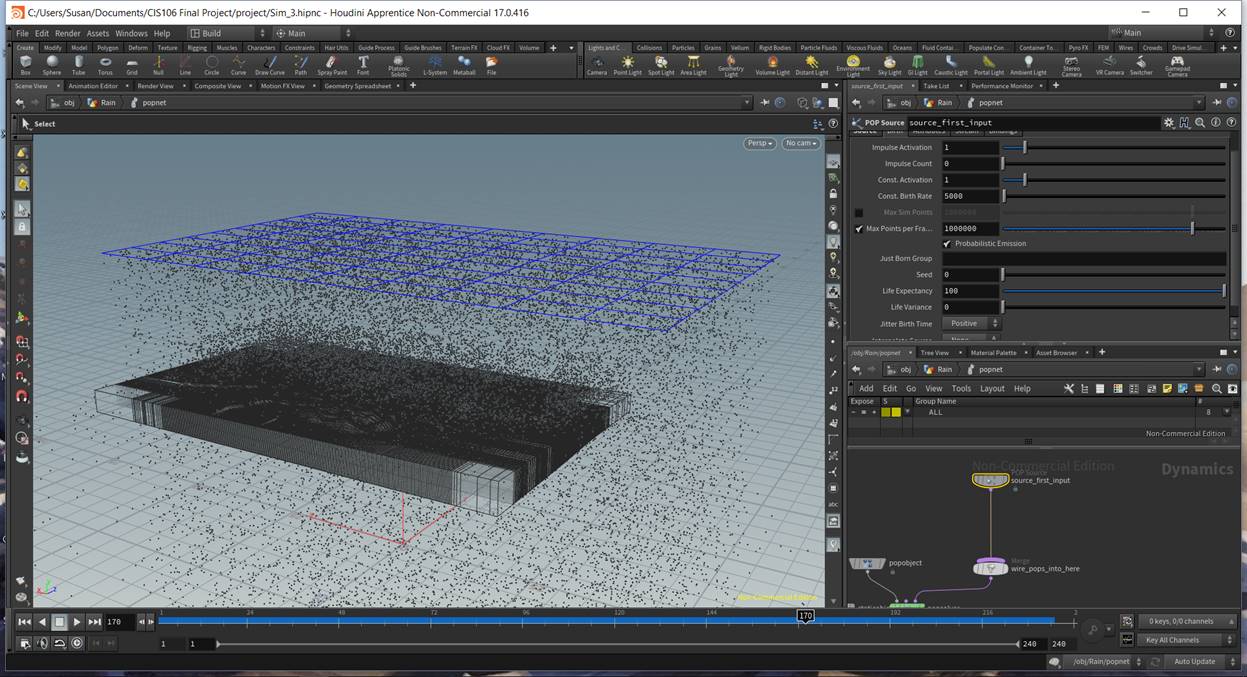
Figure 26: POPnetwork rain simulation set-up in Houdini with landscape as static object
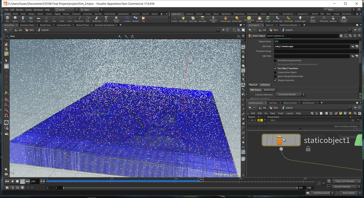
Figure 27: Rain simulation in action.
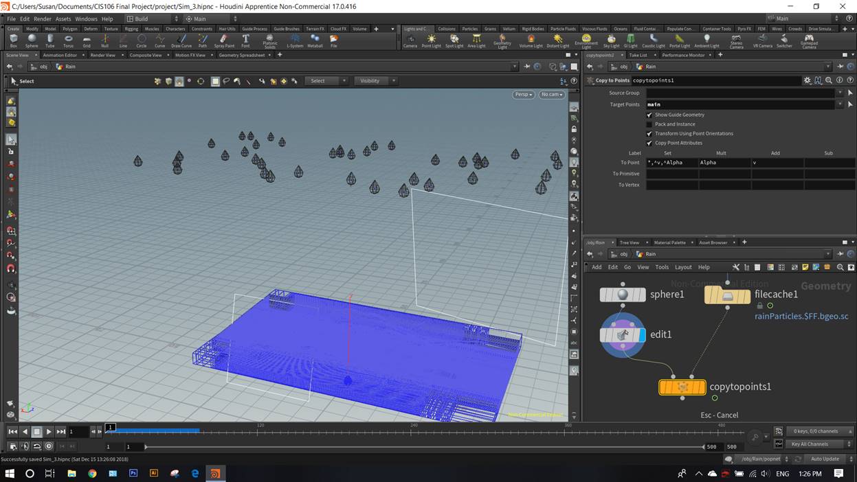
Figure 28: Geometric shape, later removed, applied to rain droplets (exaggerated).
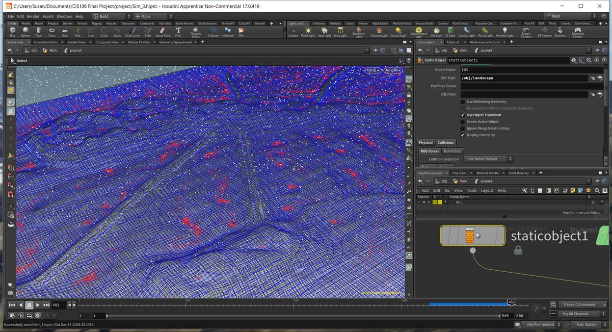
Figure 29: N“Slide” effect added to POPnetwork rain to allow for pooling of water at lower points in the mesh.
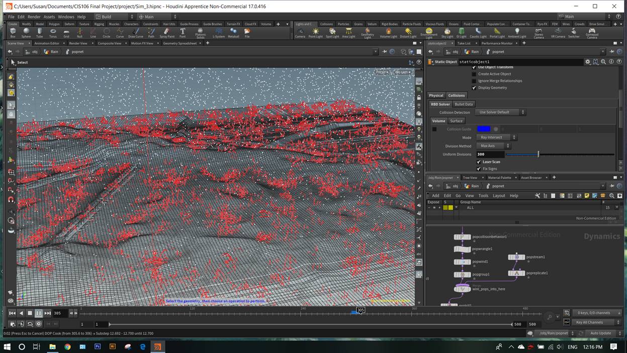
Figure 30:Splash effect added to POPnetwork rain.
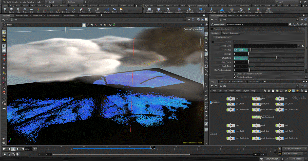
Figure 31: FLIP fluid flood simulation preview using six FLIP fluid containers.
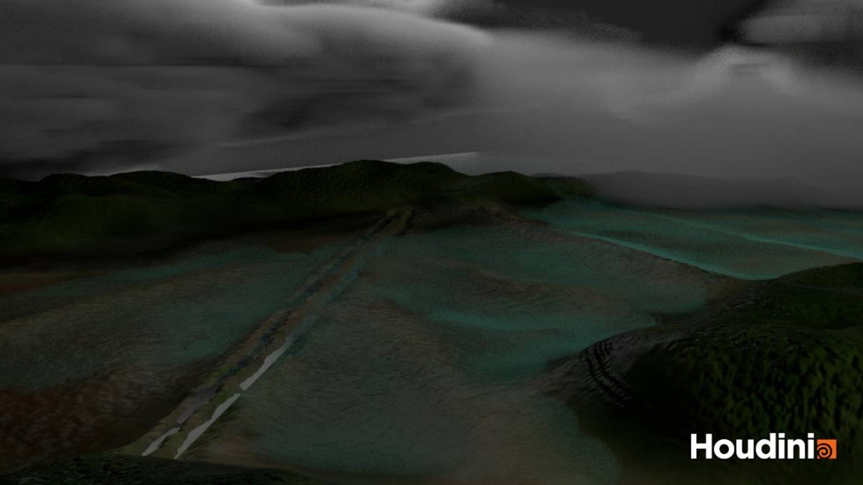
Figure 32: Dry landscape and clouds through final camera angle set-up.
Figure 33: Frame 446 from the POPnetwork rain simulationFrame 446 from the POPnetwork rain simulation
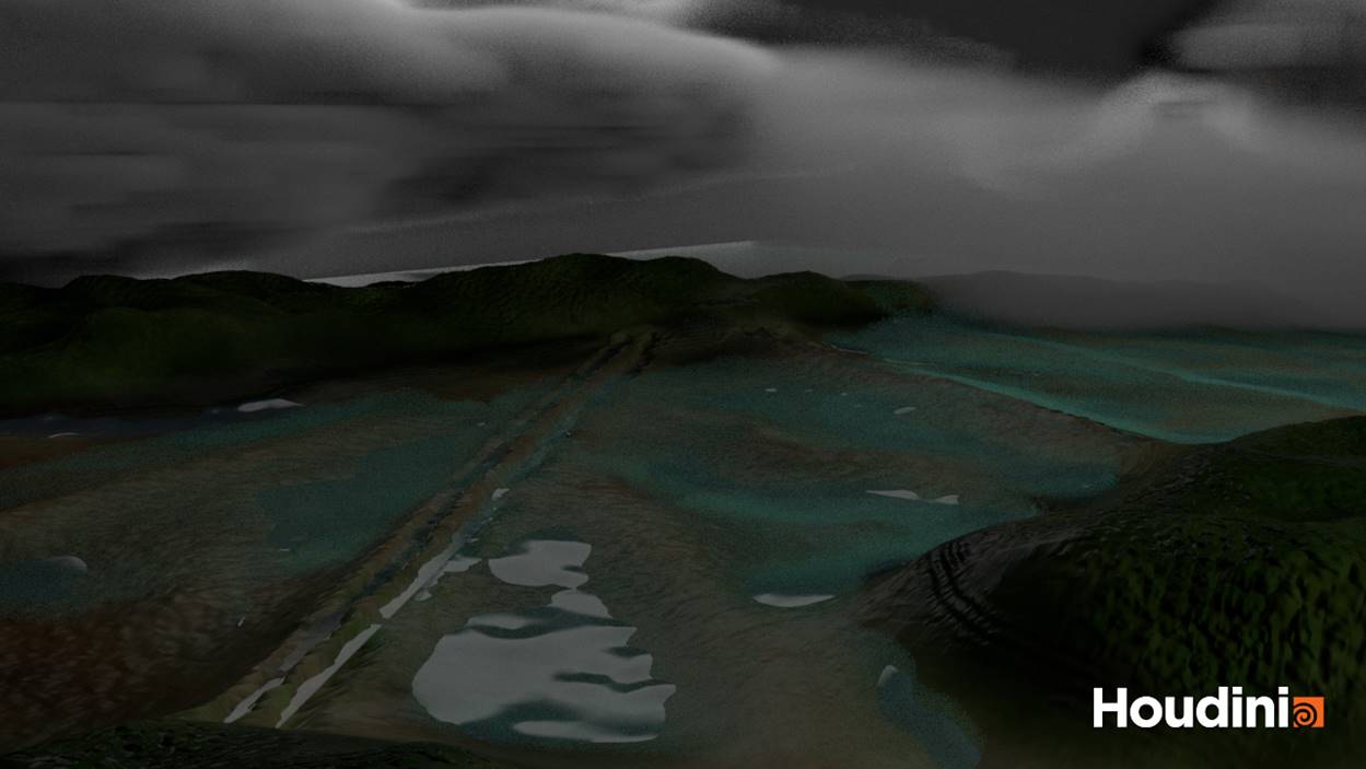
Figure 34: Level 1: low flood water level.
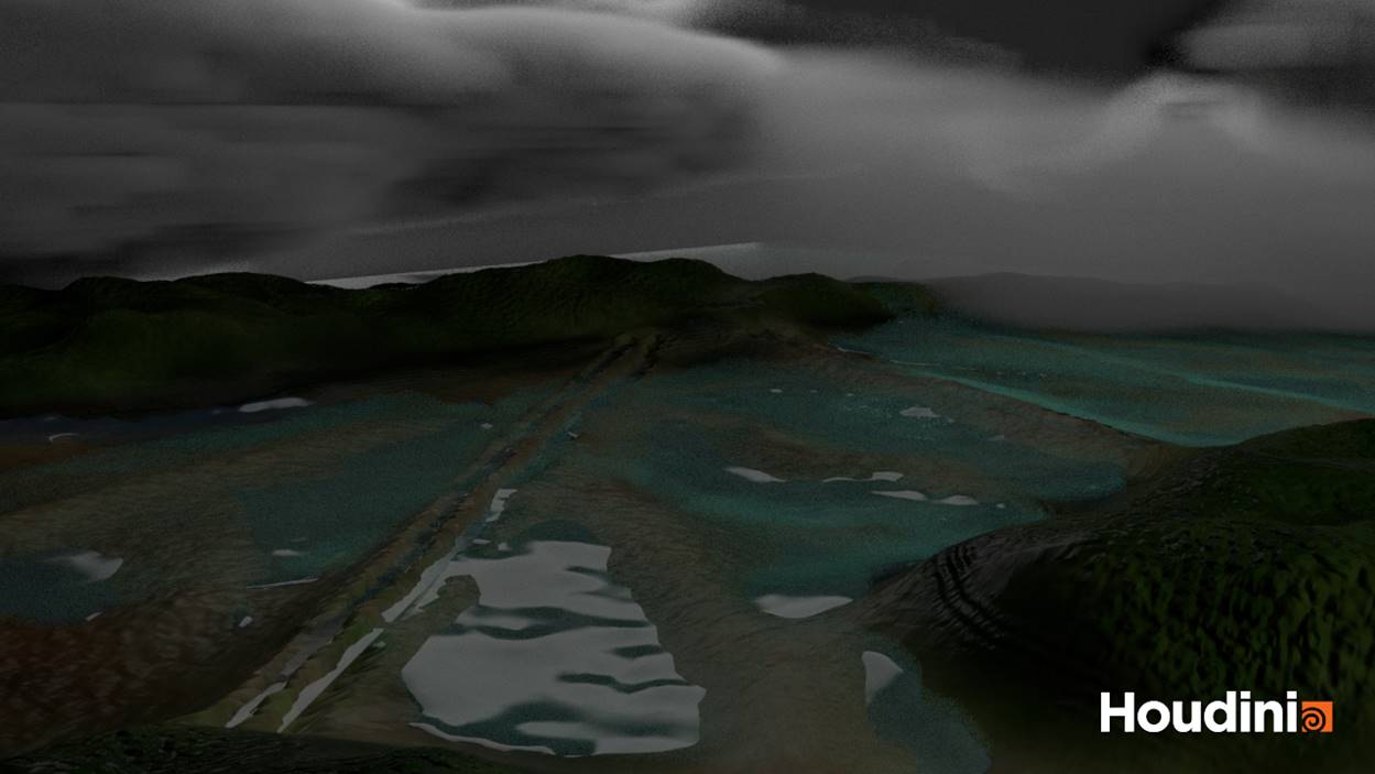
Figure 35: Level 2: lower-middle flood water level
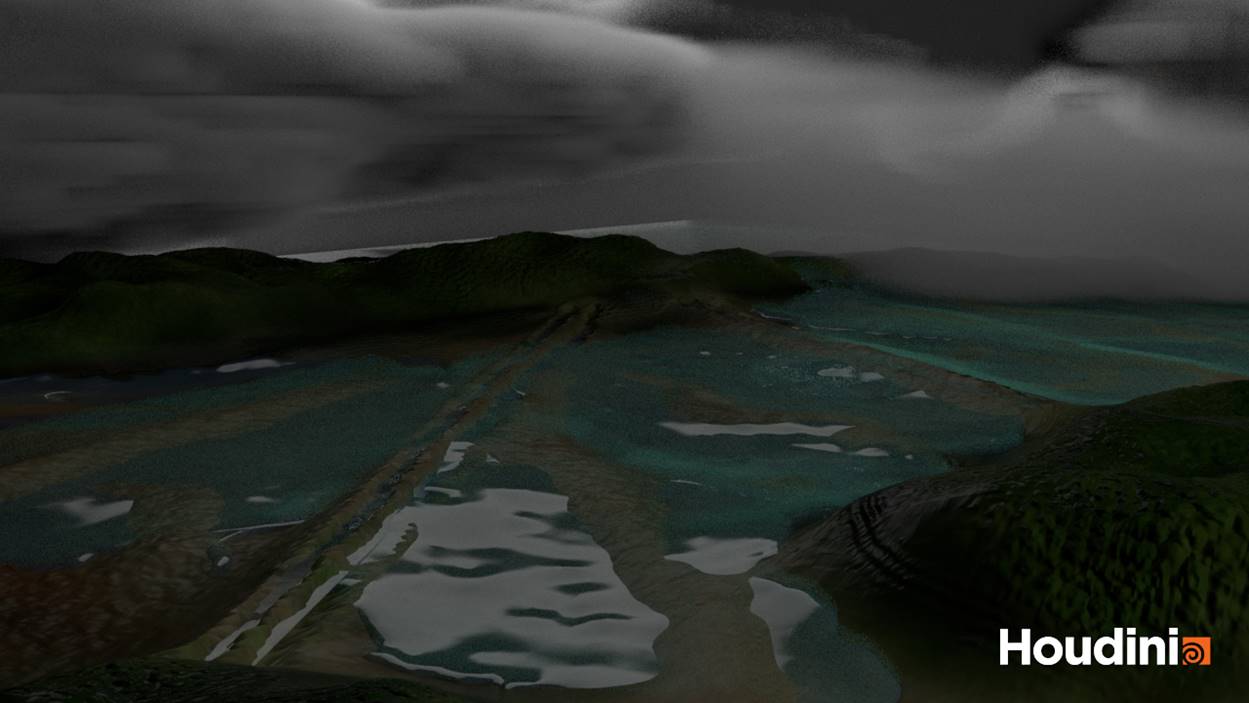
Figure 36: Level 3: middle flood water level
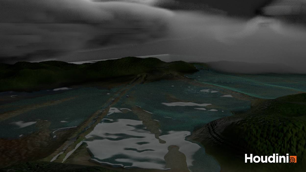
Figure 37: Level 4: upper-middle flood water level
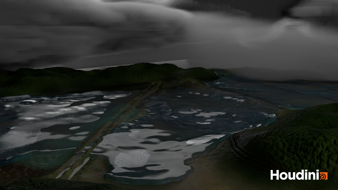
Figure 38: Level 5: high flood water level
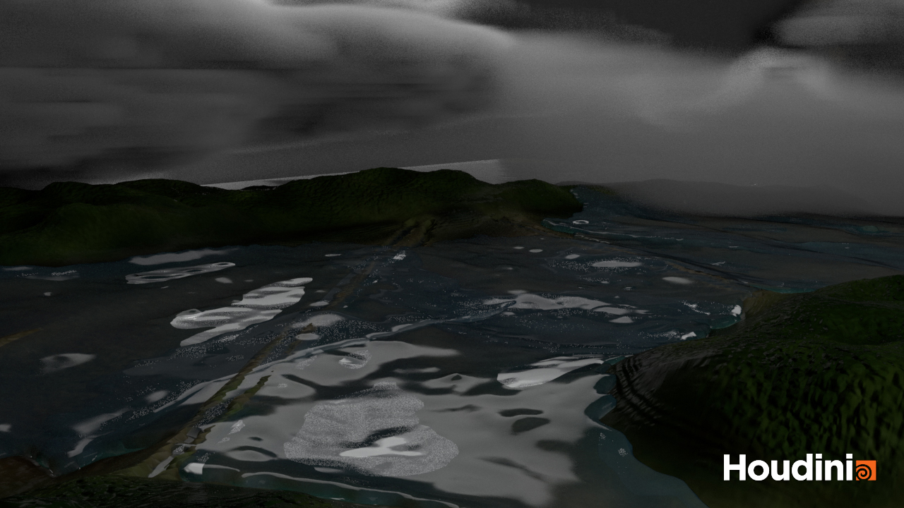
Figure 39: Level 6: highest flood water level.
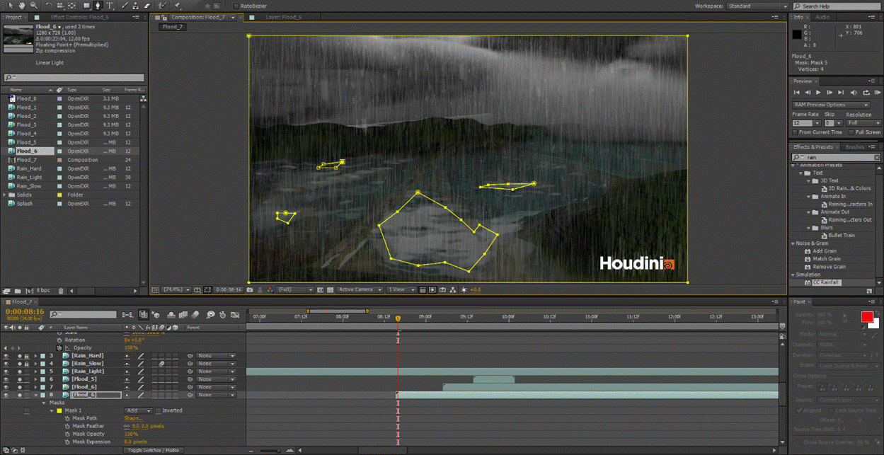
Figure 40: Timeline and mask view of wet season scene in timelapse.